[SparkML] Kaggle EDA + Regression 구현하기

- 목차

 

소개.

아래 주소는 Kaggle EDA + Regression 문제를 소개하는 페이지의 웹 링크입니다.

https://www.kaggle.com/code/hely333/eda-regression

EDA + Regression

 

위 문제에서는 메디컬 데이터가 제공됩니다.

메디컬 데이터는 환자의 상태 정보와 의료비용 데이터로 구성됩니다.

목표는 환자의 상태 데이터를 기반으로 의료비용을 예측하는 Regression 모델을 구축하는 것입니다.

 

데이터 분석하기.

import os
from pyspark.sql import SparkSession
from pyspark.sql.types import StructType, StructField, StringType, DoubleType, IntegerType

spark = SparkSession.builder.appName("eda-regression") \
    .master("local[*]") \
    .config("spark.driver.bindAddress", "localhost").getOrCreate()

file_path = os.path.abspath(os.path.join("../resources/insurance.csv"))
schema = StructType([
    StructField("age", IntegerType(), True),  # 연령
    StructField("sex", StringType(), True),  # 성별
    StructField("bmi", DoubleType(), True),  # Body Mass Index (몸무게 / 키)
    StructField("children", IntegerType(), True),  # 자녀의 수
    StructField("smoker", StringType(), True),  # 흡연 유무
    StructField("region", StringType(), True),  # 거주지역
    StructField("charges", DoubleType(), True),  # 의료비
])
medical_df = spark.read.option("header", True).csv(file_path, schema=schema)
medical_df.show()

+---+------+------+--------+------+---------+-----------+
|age|   sex|   bmi|children|smoker|   region|    charges|
+---+------+------+--------+------+---------+-----------+
| 19|female|  27.9|       0|   yes|southwest|  16884.924|
| 18|  male| 33.77|       1|    no|southeast|  1725.5523|
| 28|  male|    33|       3|    no|southeast|   4449.462|
| 33|  male|22.705|       0|    no|northwest|21984.47061|
| 32|  male| 28.88|       0|    no|northwest|  3866.8552|
| 31|female| 25.74|       0|    no|southeast|  3756.6216|
| 46|female| 33.44|       1|    no|southeast|  8240.5896|
| 37|female| 27.74|       3|    no|northwest|  7281.5056|
| 37|  male| 29.83|       2|    no|northeast|  6406.4107|
| 60|female| 25.84|       0|    no|northwest|28923.13692|
| 25|  male| 26.22|       0|    no|northeast|  2721.3208|
| 62|female| 26.29|       0|   yes|southeast| 27808.7251|
| 23|  male|  34.4|       0|    no|southwest|   1826.843|
| 56|female| 39.82|       0|    no|southeast| 11090.7178|
| 27|  male| 42.13|       0|   yes|southeast| 39611.7577|
| 19|  male|  24.6|       1|    no|southwest|   1837.237|
| 52|female| 30.78|       1|    no|northeast| 10797.3362|
| 23|  male|23.845|       0|    no|northeast| 2395.17155|
| 56|  male|  40.3|       0|    no|southwest|  10602.385|
| 30|  male|  35.3|       0|   yes|southwest|  36837.467|
+---+------+------+--------+------+---------+-----------+
only showing top 20 rows

 

제공되는 데이터의 칼럼은 다음과 같습니다.

age      : 연령
sex      : 성별
bmi      : Body Mass Index (몸무게 / 키)
children : 자녀의 수
smoker   : 흡연 유무
region   : 거주지역
charges  : 의료비

 

Categorical 데이터를 Indexer 로 변환.

sex, smoker, region 에 해당하는 categorical 데이터를 Numerical 타입으로 변환합니다.

from pyspark.ml.feature import StringIndexer, VectorAssembler

medical_df = StringIndexer(inputCol="sex", outputCol="sex_vector").fit(medical_df).transform(medical_df)
medical_df = StringIndexer(inputCol="smoker", outputCol="smoker_vector").fit(medical_df).transform(medical_df)
medical_df = StringIndexer(inputCol="region", outputCol="region_vector").fit(medical_df).transform(medical_df)
columns = [col[0] for col in medical_df.dtypes if col[1] != 'string']
assembler = VectorAssembler(inputCols=columns, outputCol="features")
medical_df = assembler.transform(medical_df)
medical_df.show()

+---+------+------+--------+------+---------+-----------+----------+-------------+-------------+--------------------+
|age|   sex|   bmi|children|smoker|   region|    charges|sex_vector|smoker_vector|region_vector|            features|
+---+------+------+--------+------+---------+-----------+----------+-------------+-------------+--------------------+
| 19|female|  27.9|       0|   yes|southwest|  16884.924|       1.0|          1.0|          2.0|[19.0,27.9,0.0,16...|
| 18|  male| 33.77|       1|    no|southeast|  1725.5523|       0.0|          0.0|          0.0|[18.0,33.77,1.0,1...|
| 28|  male|  33.0|       3|    no|southeast|   4449.462|       0.0|          0.0|          0.0|[28.0,33.0,3.0,44...|
| 33|  male|22.705|       0|    no|northwest|21984.47061|       0.0|          0.0|          1.0|[33.0,22.705,0.0,...|
| 32|  male| 28.88|       0|    no|northwest|  3866.8552|       0.0|          0.0|          1.0|[32.0,28.88,0.0,3...|
| 31|female| 25.74|       0|    no|southeast|  3756.6216|       1.0|          0.0|          0.0|[31.0,25.74,0.0,3...|
| 46|female| 33.44|       1|    no|southeast|  8240.5896|       1.0|          0.0|          0.0|[46.0,33.44,1.0,8...|
| 37|female| 27.74|       3|    no|northwest|  7281.5056|       1.0|          0.0|          1.0|[37.0,27.74,3.0,7...|
| 37|  male| 29.83|       2|    no|northeast|  6406.4107|       0.0|          0.0|          3.0|[37.0,29.83,2.0,6...|
| 60|female| 25.84|       0|    no|northwest|28923.13692|       1.0|          0.0|          1.0|[60.0,25.84,0.0,2...|
| 25|  male| 26.22|       0|    no|northeast|  2721.3208|       0.0|          0.0|          3.0|[25.0,26.22,0.0,2...|
| 62|female| 26.29|       0|   yes|southeast| 27808.7251|       1.0|          1.0|          0.0|[62.0,26.29,0.0,2...|
| 23|  male|  34.4|       0|    no|southwest|   1826.843|       0.0|          0.0|          2.0|[23.0,34.4,0.0,18...|
| 56|female| 39.82|       0|    no|southeast| 11090.7178|       1.0|          0.0|          0.0|[56.0,39.82,0.0,1...|
| 27|  male| 42.13|       0|   yes|southeast| 39611.7577|       0.0|          1.0|          0.0|[27.0,42.13,0.0,3...|
| 19|  male|  24.6|       1|    no|southwest|   1837.237|       0.0|          0.0|          2.0|[19.0,24.6,1.0,18...|
| 52|female| 30.78|       1|    no|northeast| 10797.3362|       1.0|          0.0|          3.0|[52.0,30.78,1.0,1...|
| 23|  male|23.845|       0|    no|northeast| 2395.17155|       0.0|          0.0|          3.0|[23.0,23.845,0.0,...|
| 56|  male|  40.3|       0|    no|southwest|  10602.385|       0.0|          0.0|          2.0|[56.0,40.3,0.0,10...|
| 30|  male|  35.3|       0|   yes|southwest|  36837.467|       0.0|          1.0|          2.0|[30.0,35.3,0.0,36...|
+---+------+------+--------+------+---------+-----------+----------+-------------+-------------+--------------------+

 

환자의 상태 정보와 의료비 데이터 간의 상관관계를 비교합니다.

from pyspark.ml.stat import Correlation
import numpy as np

correlation_matrix = Correlation.corr(medical_df, "features")
import seaborn as sns
import matplotlib.pyplot as plt

plt.figure(figsize=(8, 6))
correlation_np_array = np.array(correlation_matrix.collect()[0][0].toArray())
sns.heatmap(correlation_np_array,
            annot=True, cmap="coolwarm", fmt=".2f", linewidths=.5,
            xticklabels=columns, yticklabels=columns
            )
plt.title("Correlation Matrix Heatmap")
plt.show()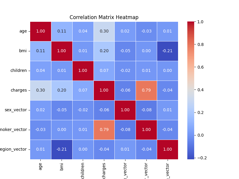

 

흡연 유무와 의료비 간의 상관관계가 비교적 큰 계수임을 알 수 있습니다.

 

 

Linear Regression 모델 구현.

from pyspark.ml.regression import LinearRegression
columns = ["age", "sex_vector", "bmi", "children", "smoker_vector", "region_vector"]
assembler = VectorAssembler(inputCols=columns, outputCol="features_vector")
medical_df = assembler.transform(medical_df)
train_df, test_df = medical_df.randomSplit([0.7, 0.3], seed=42)
regression = LinearRegression(maxIter=10000, featuresCol="features_vector", labelCol="charges")
model = regression.fit(train_df)
predictions = model.transform(test_df)
predictions.select(["charges", "prediction"]).show()

+-----------+------------------+
|    charges|        prediction|
+-----------+------------------+
|  2201.0971| 668.1669525944108|
| 18223.4512|26065.080849485203|
|7323.734819|   2898.0180294288|
| 2203.47185| 3226.959346956668|
|  1622.1885| 2657.330806401271|
|  4561.1885| 5753.144340314762|
|  2205.9808| 3851.947850259623|
| 2211.13075| 5134.818988618315|
| 36149.4835|27804.810845626533|
|  1631.6683| 5018.783212232922|
|  1631.8212| 5056.871154262468|
|  1633.9618| 5590.102342676068|
| 2217.46915|  6713.73731275209|
|  1634.5734| 5742.454110794237|
| 38792.6856|29671.120005074124|
| 12829.4551|22764.999190806666|
|  1702.4553|-80.02259010475973|
| 1704.70015| 479.1776496926195|
|  1705.6245| 709.4365719621273|
|15518.18025| 24445.93148600206|
+-----------+------------------+